Viewing your data
Now we have become acquainted with our working directories and the R environment, its time to explore our newely imported data. For this, we will be using the weeds dataset. Ensure your data is loaded in and then either use the View() command:
weeds <- read.csv("weeds.csv")
View(weeds)
# This will open up a new tab to view your data
or click the variable name in the environment window.
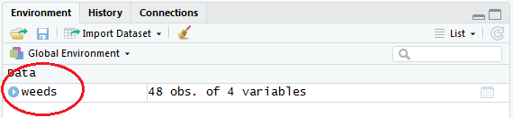
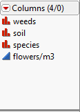
This should bring up a separate tab in Rstudio which you should be able to see the 4 columns (weeds, soil, species & flowers.m3).
Now we can see our data, we can investigate the way R has input our data. The best thing to do is to ensure your categorical variables are categorical, and our continuous are continuous, much like we do in programs like JMP.
In JMP, we have the icons to identify categorical/nominal, ordinal or continuous. In R, all we do is run a single line of code to view the same thing across the different columns.
str(weeds)## 'data.frame': 48 obs. of 4 variables:
## $ weeds : Factor w/ 2 levels "native","weed": 2 2 2 2 2 2 2 2 2 2 ...
## $ soil : Factor w/ 2 levels "sandstone","shale": 1 1 1 1 1 1 1 1 1 1 ...
## $ species : Factor w/ 3 levels "Coprosma","Olearia",..: 1 1 1 1 3 3 3 3 2 2 ...
## $ flowers.m3: int 14 17 23 26 35 45 36 28 28 39 ...# str stands for "structure" and will tell us the formats of each data column, as well as the number of levels when we have a factor (categorical) columnstr() also shows us the number of levels we have in a factor. So if we put in a bad dataset with different capitalisations or misspellings on factor levels, we can identify here how many we want vs. how many we have. Its a quick and easy way to assess your data.
As you can see in the weeds example, we have weeds, soil & species as factors (categorical) and flowers.m3 as an integer (one of many continuous data types, in this case, whole numbers).
We will follow up on how to fix an incorrect column shortly
Other data viewing commands can be used to view certain aspects of your data without bringing up the entire data set in a new tab. These are as follows:
head(weeds) # This will show the top few rows of your data so you can check it without loading the entire table## weeds soil species flowers.m3
## 1 weed sandstone Coprosma 14
## 2 weed sandstone Coprosma 17
## 3 weed sandstone Coprosma 23
## 4 weed sandstone Coprosma 26
## 5 weed sandstone Pultenaea 35
## 6 weed sandstone Pultenaea 45tail(weeds) # The same as head() but shows the bottom rows## weeds soil species flowers.m3
## 43 native shale Pultenaea 49
## 44 native shale Pultenaea 20
## 45 native shale Olearia 32
## 46 native shale Olearia 51
## 47 native shale Olearia 47
## 48 native shale Olearia 55dim(weeds) # This gives you the number of rows and columns## [1] 48 4# You can also use nrow(weeds) or ncol(weeds) to get them separately
names(weeds) # Gives you the column names. ## [1] "weeds" "soil" "species" "flowers.m3"# I use this when I want the exact name for a column when I am writing analyses (you will see later how useful this can be)
summary(weeds) # Gives you summary statistics for each column## weeds soil species flowers.m3
## native:24 sandstone:24 Coprosma :16 Min. :13.00
## weed :24 shale :24 Olearia :16 1st Qu.:22.50
## Pultenaea:16 Median :33.00
## Mean :33.81
## 3rd Qu.:45.50
## Max. :57.00# This will also come in handy later for statistical analysis As you can see, there are many ways to view data within R. Some of these are useful for huge datasets (> 10k rows) as the view() command can put strain on your computer. Using head() or tail() to view aspects of the data is useful as it reduces how much is displayed.
After reading in dataset, use the summary() command with the “insecticide”” dataset to answer the following questions:
Question: What is the minimum value for species richness?
Question: What is the maximum value for species richness?