Basic plots
To start, we will use the iris dataset that is built into tidyverse/ggplot2. To view the dataset, use the View() command like so:
View(iris)Once we have this, let’s setup a basic boxplot of some of the features of iris.
The iris dataset is built into tidyverse/ggplot2. The dataset is a pretty famous dataset by Edgar Anderson that gives the sepal length, width and petal length and width for three species of iris (n=50).
We are going to begin by plotting the sepal length for each species in a basic boxplot.
iris.box <- ggplot(iris, aes(x=Species,y=Sepal.Length)) +
geom_boxplot()
iris.box # We have to run a line with the name of the plot object to view the graph. 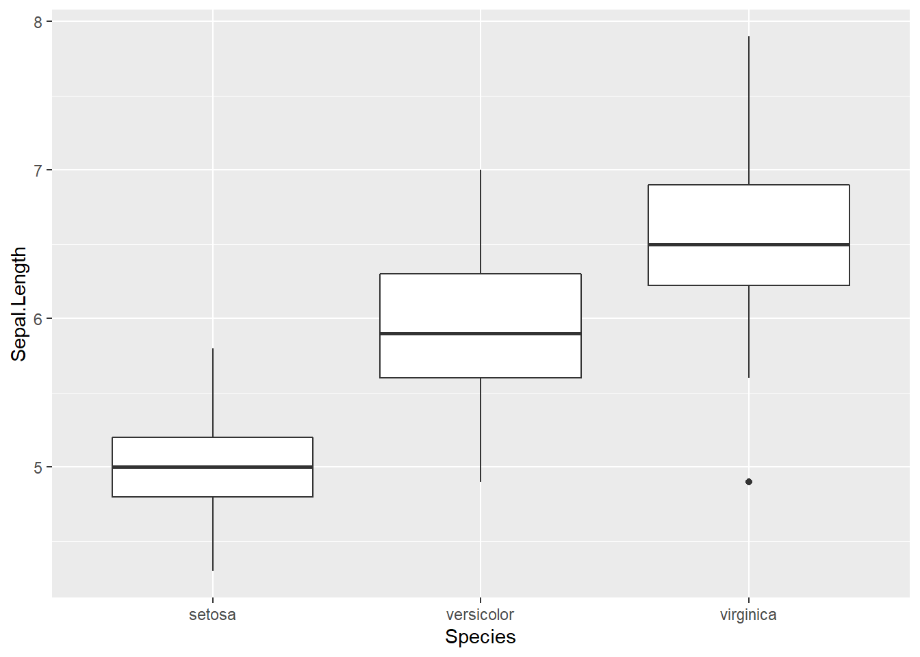 So far, pretty straight forward.
You will notice I saved the ggplot() graph to an object called iris.box. Because I saved the plot to an object, I have to run the object name to view the plot. This is identical to using the command print(iris.box).
ggplot graphs do no need to be saved as an object. You can run all of the commands singularly or as a group. The graph will still be produced. I personally prefer to save them to an object.
Now let’s look at some others, such as a histogram.
iris.hist <- ggplot(iris, aes(x=Sepal.Length)) +
  geom_histogram()

iris.hist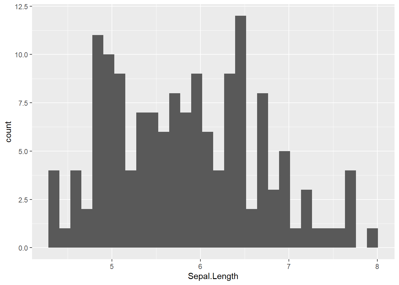
That’s pretty ugly, but a simple addition of binwidth=“value” will fix that. Binwidth refers to the width of each bin, or bar, in the frequency histogram. A bin width of 0.5 means each bar of the histogram will be equal to 0.5 on the x axis (e.g. 4, 4.5, 5, 5.5 etc).
iris.hist <- ggplot(iris, aes(x=Sepal.Length)) +
  geom_histogram(binwidth = 0.5)

iris.hist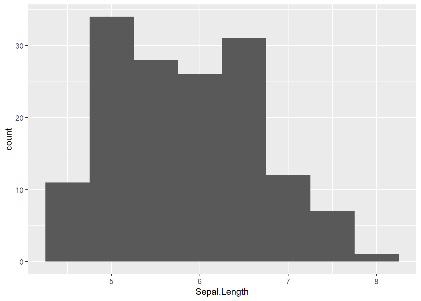
Now let’s look at a scatterplot.
iris.scatter <- ggplot(iris, aes(x=Sepal.Length,y=Petal.Length)) +
  geom_point()

iris.scatter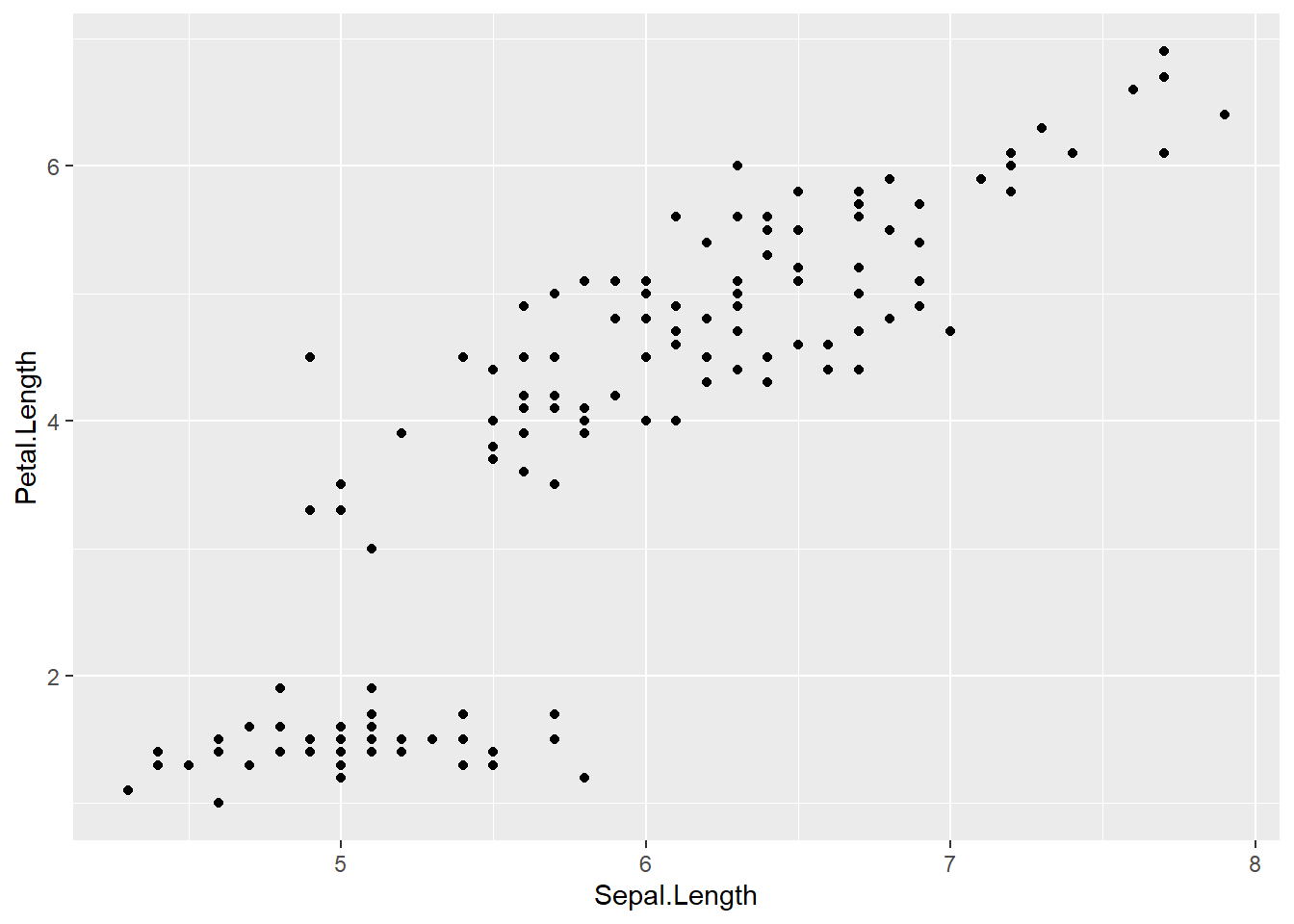
The cool thing we can do with scatterplots is colour the points by a categorical feature such as Species. This is done by adding colour = “categorical variable name” in the aes brackets of the ggplot() command.
iris.scatter <- ggplot(iris, aes(x=Sepal.Length, y=Petal.Length, colour=Species)) +
  geom_point()
iris.scatter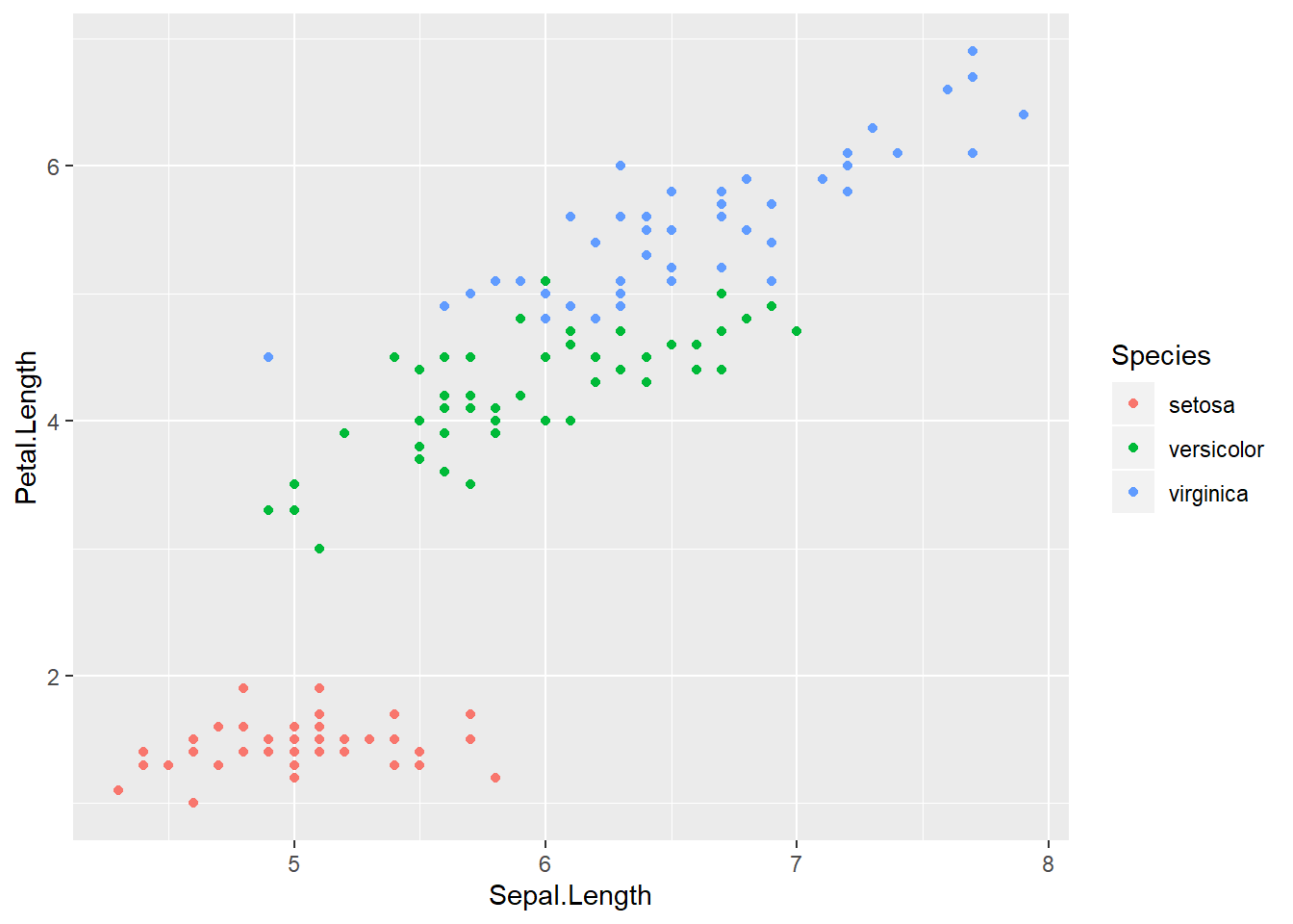
Much better. And it even adds a legend for us.
Now we have this basic setup, we can start adding things to our graph. Due to the immense amount of customisations for our graphs, I will break these down in to sections as much as possible and explain as I go. We will work with the iris dataset for a while before moving to our analysed datasets.