Linear Regression
Linear regression is one of the most highly used statistical techniques in all of life and earth sciences. It is used to model the relationship between a response (Y) variable and a explanatory (X) variable. A linear regression is a special case of a linear model whereby both the response and explanatory variables are continuous. The ANOVA we just conducted is still considered as a linear model since the response variable is a linear (additive) combination of the effects of the explanatory variables.
Since we have already conducted an ANOVA, a linear model will be a peice of cake!
For this, we will be using the tadpoles.csv dataset.
str(tadpoles) # three columns, all continuous## 'data.frame': 24 obs. of 3 variables:
## $ reeds : int 1 1 1 1 1 1 1 1 2 2 ...
## $ pondsize : int 45 60 20 45 56 16 37 49 50 16 ...
## $ abundance: int 120 201 136 128 178 55 156 150 89 25 ...Automatically, upon reading the tadpoles dataset, we have an issue. Our reeds column should actually be a category, so we need to read that in as a factor. There is argument here for reeds to be ordinal, but for ease of interpretation, we will stick to just a factor.
Make reeds into a factor
Once everything is input correctly, we can begin our analysis
tadpoles.lm <- lm(abundance ~ pondsize, data = tadpoles) # constructing a linear modelThe lm() command creates a linear model object. In this example we are testing the effect of pondsize on tadpole abundance using a linear regression.
It is worth noting that the lm() command can be used to perform an anova, but the aov() command cannot be used for regressions. Give it a try by using lm on our last analysis and use the anova command, as well as the summary() command on the created object.
summary(tadpoles.lm) # summarising the newly created linear model object##
## Call:
## lm(formula = abundance ~ pondsize, data = tadpoles)
##
## Residuals:
## Min 1Q Median 3Q Max
## -73.546 -29.752 -8.026 37.978 77.652
##
## Coefficients:
## Estimate Std. Error t value Pr(>|t|)
## (Intercept) 23.8251 25.8455 0.922 0.36662
## pondsize 1.7261 0.5182 3.331 0.00303 **
## ---
## Signif. codes: 0 '***' 0.001 '**' 0.01 '*' 0.05 '.' 0.1 ' ' 1
##
## Residual standard error: 49.42 on 22 degrees of freedom
## Multiple R-squared: 0.3352, Adjusted R-squared: 0.305
## F-statistic: 11.09 on 1 and 22 DF, p-value: 0.003032The estimates for the coefficients give you the slope and the intercept (much like JMP). In this example, the regression equation would be:
Abundance = 23.8251 + 1.7261*pondize + error The summary() printout gives us a lot of useful information, so we need to narrow down what is most important. The t-value and p-value for each coefficient indicate significance. We dont really care about the intercept. What we do care about is if the other coefficient (pondsize) is significant, indicating an effect of the explanatory variable on the reponse. Because of the positive estimate (1.7261) we can identify that an increase in pondsizeis associated with a significant increase in tadpole abundance.
While the t and p-values indicate a significant association, the R^2 value tells us the strength of the association. In this case, the proportion of variation explained by the explanatory variable is 33.52%.
Assumptions
To test assumptions for linear regression, we need to test the same assumptions we tested for the ANOVA. The only slight exception here is the pattern/appearance of the residuals in the fitted v.s residuals plot AND, we cant use bartlett’s or levene’s tests.
plot(tadpoles.lm, 1)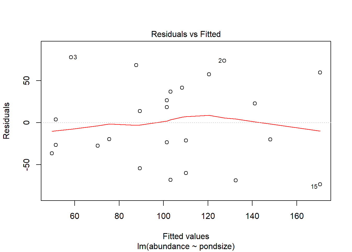
In this plot we are looking for an even “shotgun” like appearance in the residuals. We want an even dispersal around the grand mean. In this example, we have a spread of redisuals that does not appear to follow any non-linear trends. There is no point trying to fit a straight line through data that is curved. If there is strong patterning in your residuals, try log-transforming your response or, fit a polynomial function (e.g. quadratic).
Click the link below to see a nice interactive app that demonstrates what patterns of residuals you would expect with linear and curved relationships:
Linear regression diagnostics https://gallery.shinyapps.io/slr_diag/
Test your normality before moving on.