Saving multiple figures
While facetting is useful, sometimes we need to save multiple different plots into one image. There are a number of ways to accomplish this and each have their benefits.
This section will only cover the “ggpubr” package. This is my personal choice for combining plots and accomplishes everything I need for publication quality figures. It should be noted that there are a plethora of packages that all accomplish a similar task (e.g. “cowplot”, “grid” and “gridExtra”) each with their own unique features and syntax.
For these examples, we will be using the weeds datasets, producing 2 graphs, one with species on the x-axis and one with soil, just to demonstrate this usage in a publication setting. I have already setup each of the graphs separately, using similar code as the bargraph tutorials, just changing the x-axis (for the most part).
ggpubr is a popular solution, particularly for those utlising ggplot2 for their plotting needs. The main feature from this package is ggarrange() which will help arrange plots and allows further customisation in removing labels (for shared x or y axes), combining legends and even labelling each plot.
Let’s start with an example
library(ggpubr)
ggarrange(weeds.bar.species, weeds.bar.soil, ncol = 2, nrow = 1)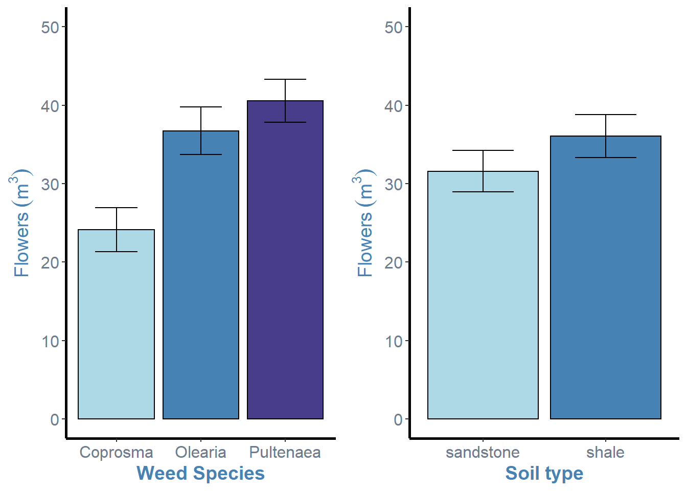
For this function, we simply specify the different ggplot objects in order, followed by the number of columns (ncol) and numebr of rows (nrow). This function is awesome at aligning axes and resizing figures.
From here, we can simply save the arranged plot using ggsave().
When saving figures, I tend to assign the figure to an object so I know ggsave() is using that object
arrange <- ggarrange(weeds.bar.species, weeds.bar.soil, ncol = 2, nrow = 1)
ggsave("arrangedplot.png", arrange)
Removing axes labels
The most obvious modification we can make to these arranged plots is the removal of the shared y-axis label. This is very simple.
ggarrange(weeds.bar.species, weeds.bar.soil + rremove("ylab"), ncol = 2, nrow = 1)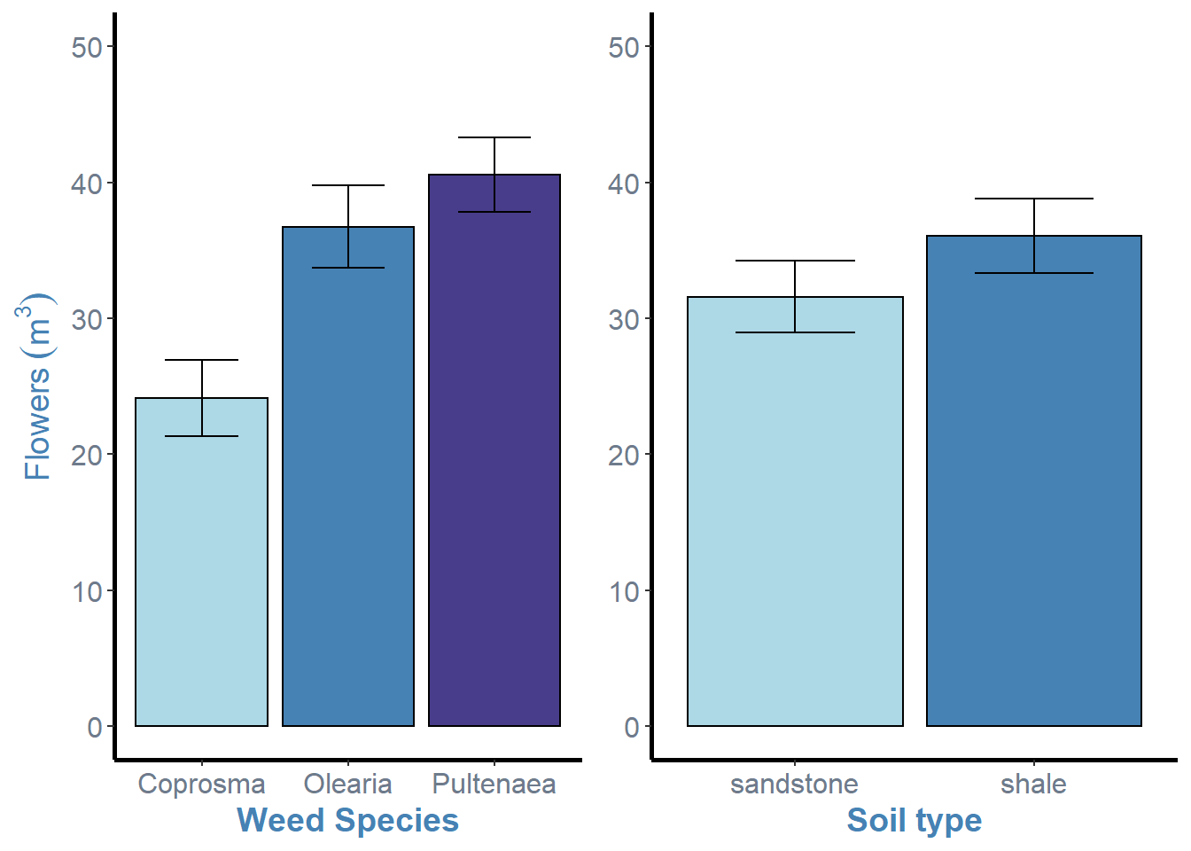
In this example, all we need to do is simply add the rremove() argument to one of the plot objects and specify what feature we wish to remove, in this case the “ylab” or y axis label.
Adding plot labels
The next feature most people will need when combining multiple plots together is labelling each plot with a letter in order to refer to a specific figure in text or in the caption. Again, this is really easy and just requires a single addition to our ggarrange().
ggarrange(weeds.bar.species, weeds.bar.soil, ncol = 2, nrow = 1, labels = "AUTO")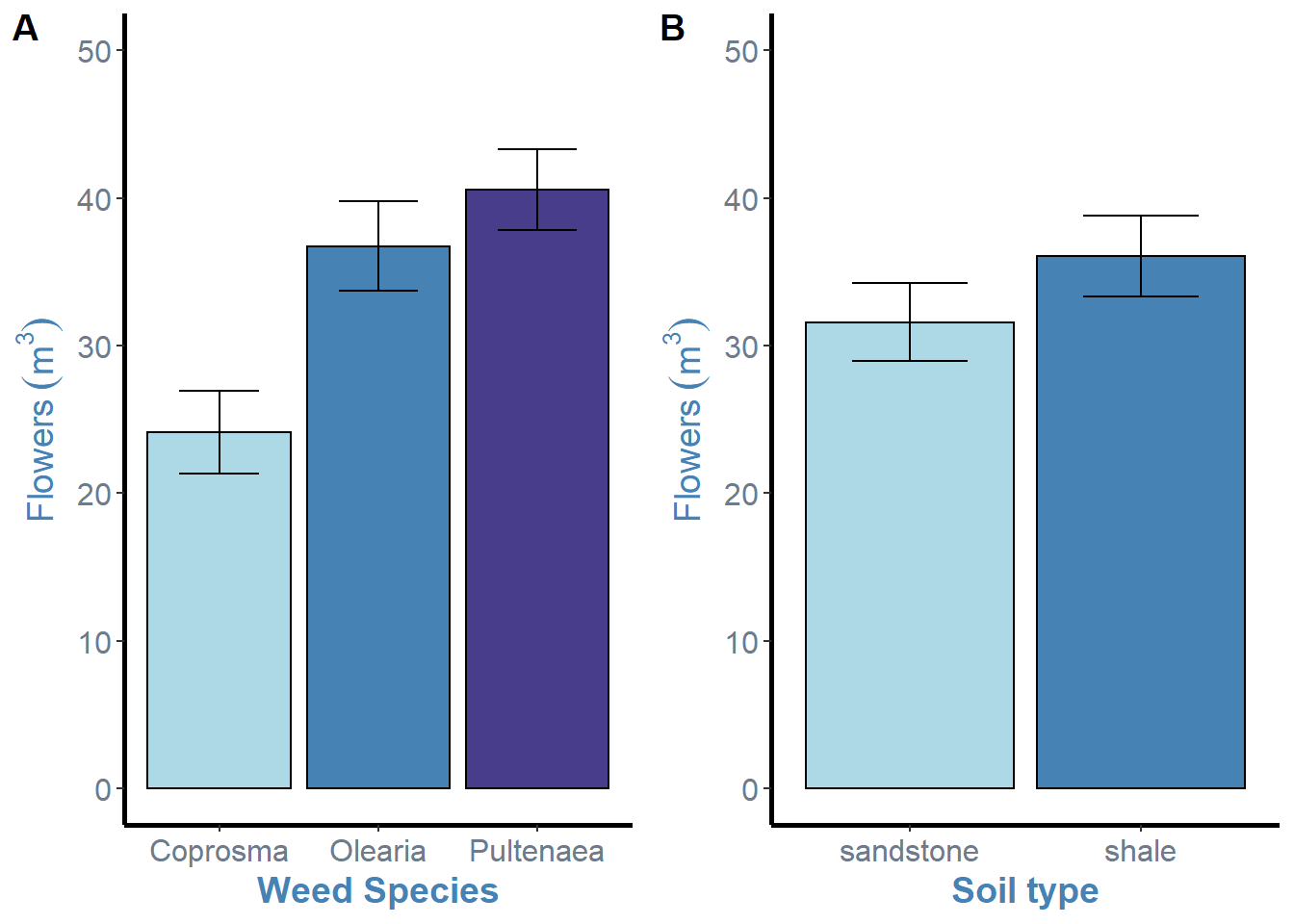
ggarrange() simply needs the “labels” argument to add to each of the plot.
These can be specified using “AUTO” for automatic uppercase lettering, or “auto” for automatic lower case lettering. Alternatively, you can specify your own custom letters using c(“A”, “B”) specifying your labels inside the concatinated brackets.
You may have noticed that I removed the rremove() command during that last ggarrange. This is due to the way ggarrange() places its labels. To fix this, we can add the hjust = argument to our function, but its a little annoying.
# Default with no hjust
ggarrange(weeds.bar.species, weeds.bar.species + rremove("ylab"), ncol = 2, nrow = 1, labels = "AUTO") 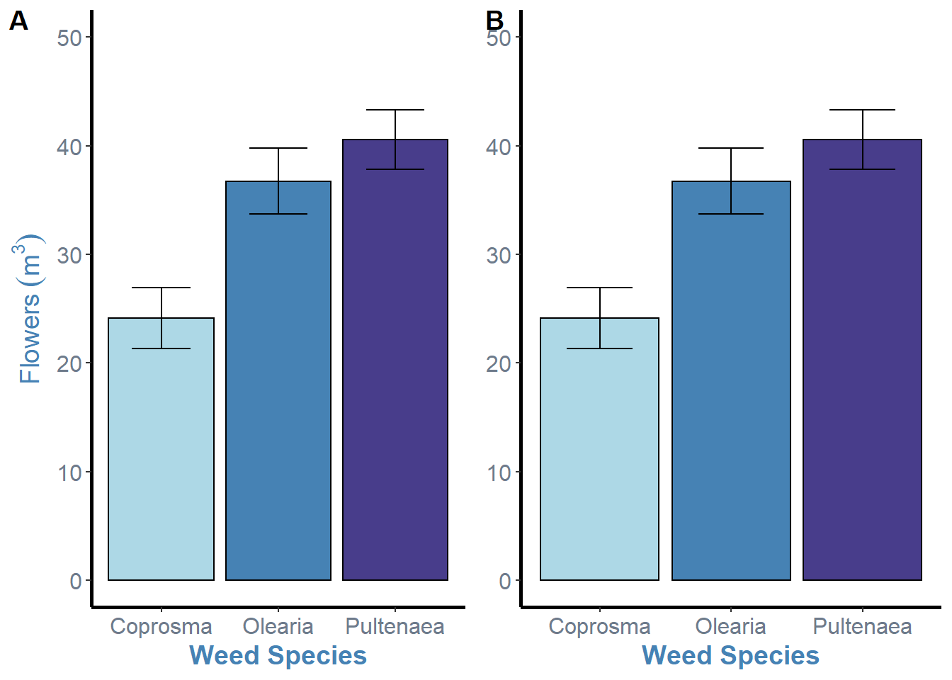
# Changing the horizontal position of the labels
ggarrange(weeds.bar.species, weeds.bar.species + rremove("ylab"), ncol = 2, nrow = 1, labels  = "AUTO", hjust = c(-5, -2.5))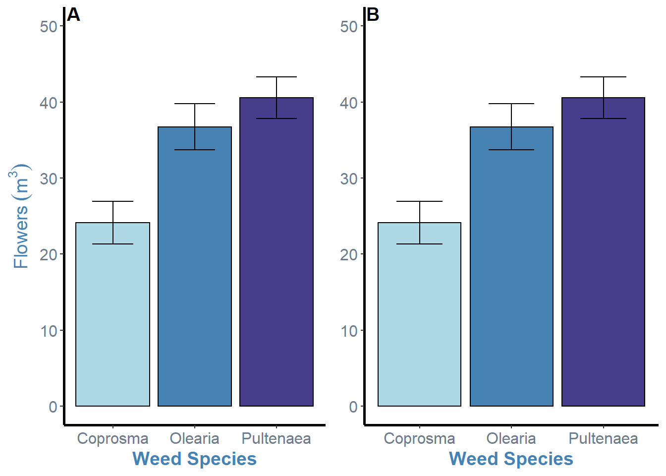
This isnt the most elegant solution, but its my sure fire way to fix the issue and also put the label inside the plot which I prefer. This is just the addition of the hjust = argument and changing the horizontal position for each plot inside the c() brackets. The values here were just through trial and error. Negative values will move the labels to the right, so the first plot needs a higher value due to the y axis label space it needs to overcome.
After all of this, we can save our “final” figure.
arrange <- ggarrange(weeds.bar.species, weeds.bar.species + rremove("ylab"), ncol = 2, nrow = 1, labels  = "AUTO", hjust = c(-5, -2.5))

ggsave("arrangedplot.png", arrange, width = 8, height = 6)
References:
Statistical tools for high-throughput data analysis - ggpubr publication ready plots