Facetting
Facetting is the process of dividing a plot into subplots based on the values of a discrete variable. In the context of the Iris scatterplots, we can split by species across multiple plots.
ggplot(iris, aes(x=Sepal.Length, y=Petal.Length)) +
  geom_point() +
  facet_grid(.~Species)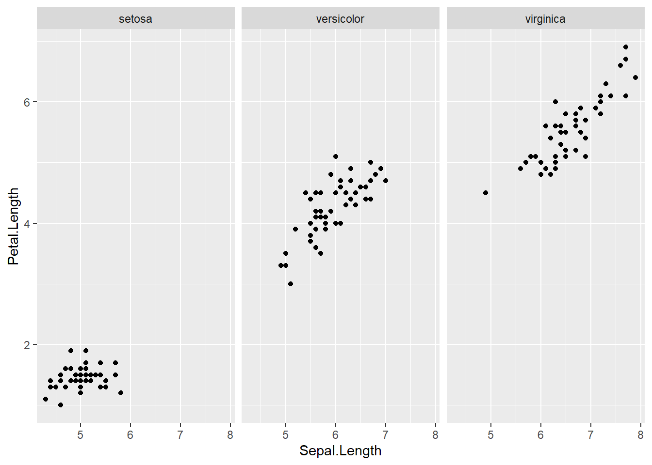
As you can see, facet_grid() splits our single plot into a number of plots equal to the levels of the factor we specify. The syntax behind facet_grid() specifies our “rows” and “columns” for our plots separated by a ~ tilde. E.g. facet_grid(row~column).
If we dont have a factor for one of the column/row arguments, we just place a full stop.
A better example of this is using facet_wrap() with our weeds bar graph. facet_wrap() sorts the graphs into a rectangular layout by default.
weeds.bar2 <- ggplot(weeds.summarise2, aes(x=species, y=mean, fill=species))+
  geom_bar(stat="identity", show.legend=F, colour="black")+
  labs(x="Weed Species", y= expression(Flowers~(m^3)))+
  theme(panel.background = element_blank(), panel.grid = element_blank(), axis.line = element_line(colour = "black", size=1), axis.text = element_text(colour="lightsteelblue4", size=12), axis.title = element_text(colour="steelblue", size=14, face="bold"))+
  scale_fill_manual(values = c("lightblue", "steelblue", "darkslateblue"))+
  geom_errorbar(aes(ymin = mean-se, ymax = mean+se), width=0.5)+
  ylim(0, 50)+
  facet_wrap(~soil)

weeds.bar2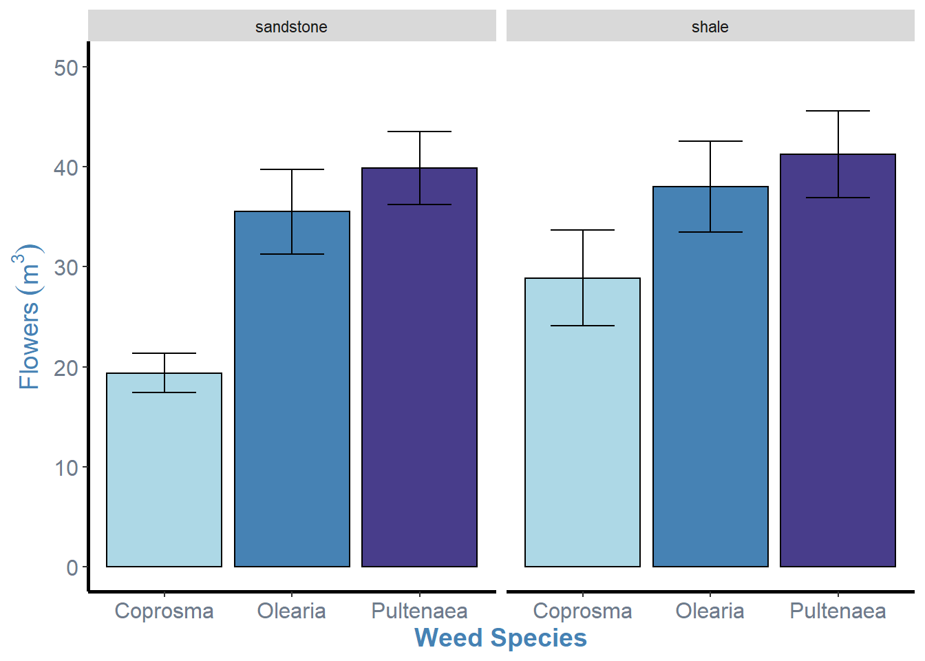
As you can see, we have facetted by soil, creating two bar graphs of species by flowers, for each level of soil.
With facet_wrap() we only specify one variable. This is useful for factors with many levels as it will automatically wrap to multiple rows. That is to say, instead of having 5 plots in a single row it might place 3 in the top row and 2 in the bottom.